Consumption Analytics
Full analysis of a single gas metering node — data quality, consumption profile, device passport and event journal, with optional forensic detail.
Consumption Analytics is a detailed metrological and operational deep-dive into one gas metering node over the selected period. The goal is not just to draw a consumption chart, but to answer the practical questions of the metering service. The analysis applies international metrology references where they justify a number: ISO 5167 (orifice metering), EN 12405-1 (electronic volume conversion devices), OIML R 137 (gas meters), OIML R 140 (measuring systems for gaseous fuel), ISO 6976 (calorific value), EN 1359 (diaphragm gas meters) and EN 14236 (ultrasonic domestic gas meters).
Purpose

Report header. The first thing the reader sees: node name and address, corrector type, last-hour key metrics (P, T), total data volume in the window (points), number of detected events, analysis method (rules / rules+LLM / LLM-only), fetch duration and the covered period.
The report answers the metering service’s day-to-day questions:
- is the data for the selected period complete;
- can the archive be used for commercial period closure;
- is there a tail gap at the end of the period;
- is current telemetry working;
- does hourly flow match the cumulative volume;
- are any P/T sensors stuck;
- are there communication or archive-delivery issues;
- is the metrology passport sufficiently filled;
- are there suspicious under-metering patterns;
- is a site visit needed;
- which role should act: metrologist, dispatcher, comms engineer, integration engineer, field crew or billing analyst.
Core logic
The report separates three orthogonal assessments that must not be mixed:
| Assessment | Meaning |
|---|---|
| Period data readiness | is the archive usable for the selected period |
| Current telemetry status | is the node alive at the moment of report generation |
| Commercial-closure readiness | can the period be used for billing without manual reconciliation |
A historical period can be perfectly usable for analysis even if the node is silent today.
Example of correct interpretation:
Period data:           usable with caveats
Current monitoring:    degraded
Billing closure:       not ready for final closure
This is not a contradiction. It means: historical data is partially usable, but current telemetry or commercial closure needs additional verification.
Glossary
| Term | Meaning |
|---|---|
| Q | hourly flow, m³/h |
| P | gas pressure, kPa |
| T | gas temperature, °C |
| V | cumulative volume, m³ |
| ΣQ | sum of hourly flows over the period |
| ΔV | cumulative volume increment over the period |
| H_expected | how many hours were due in the reporting period |
| H_received | how many hourly records were actually received |
| H_validQ | how many records have a valid flow value |
| H_nullQ | how many records exist but with a NULL flow |
| H_missing | how many hours are absent from the archive |
| final_tail_gap | absence of data at the end of the period |
| internal_gap | gap inside the period |
| freshness | how current the last archive hour is |
| passport completeness | metrology passport fill rate |
| incident | a grouped issue requiring action |
Analysis time window
Period start and end
You set the period start and end. The report analyses every hour from the first day’s 00:00 to the last day’s 23:00:
Expected number of hours
For a yearly period typically .
Archive availability breakdown
| Category | Meaning |
|---|---|
| Valid hour | record exists with a correct flow value |
| NULL hour | record exists but flow is empty |
| Internal gap | hour missing inside the period |
| Tail gap | missing hours at the end of the period |
| Unobserved hour | any hour without a valid flow value |
Formulas:
Data completeness
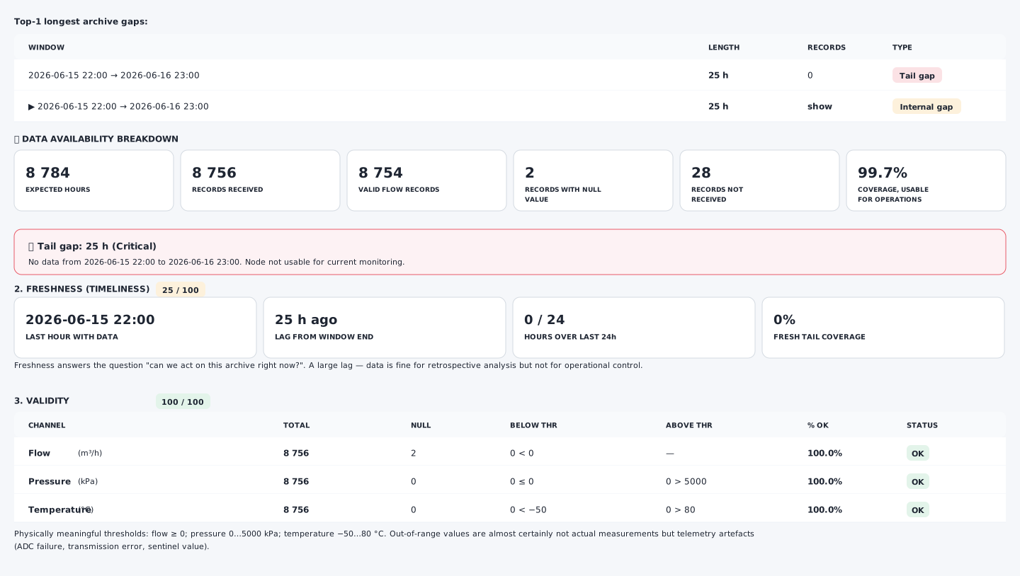
Availability, freshness and validity are three orthogonal slices in the archive-fitness check before any substantive analysis. Completeness answers: how many hours of the expected ones arrived. Freshness — how up-to-date the data is right now. Validity — whether values fall into physically reasonable ranges.
Coverage formula
Additionally:
The difference matters:
Coverage_received— whether the records arrived at all;Coverage_valid— whether they are usable for flow analysis.
Coverage interpretation
| Coverage | Status | Meaning |
|---|---|---|
| ≥ 98 % | Excellent | archive nearly complete |
| 95–98 % | Good | usable with minor caveats |
| 80–95 % | Warning | noticeable gaps |
| 50–80 % | Major | manual reconciliation required |
| < 50 % | Critical | not usable for most tasks |
Tail gap
Tail gap = absence of archive data at the end of the selected period.
| Tail | Status |
|---|---|
| ≤ 2 h | acceptable |
| 2–6 h | warning |
| 6–24 h | major |
| > 24 h | critical |
| > 168 h | device silent for over a week — urgent site visit |
The tail gap answers: can the period be considered fully closed? If data is missing at the end, the report may still be usable for retrospective analysis but is not ready for final commercial closure (see Commercial Metering Verdict).
Data freshness
Two separate freshness metrics.
Freshness vs end of period
Used for historical analysis and billing:
Answers: is there data up to the end of the selected period?
Freshness vs generation moment
Used for current monitoring:
Answers: is the node alive right now?
Coverage of last 24 hours
Composite freshness score
Current telemetry status
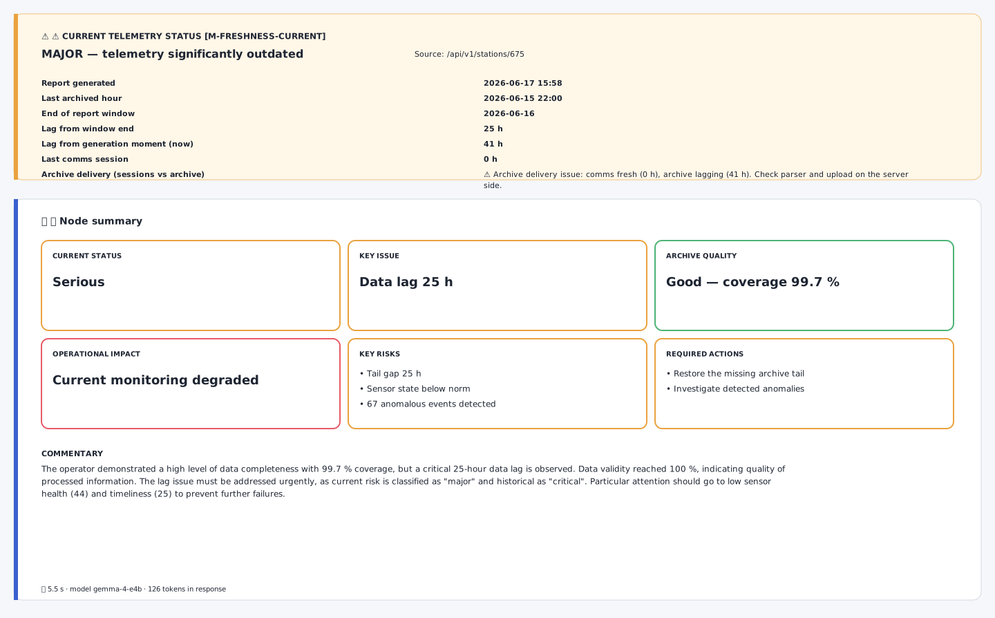
Current monitoring and node summary. This block answers “can we act on this archive right now?”. Three moments are compared: the last archived hour, the end of the reporting window, and the report-generation moment. If comms are fresh but archive lags — the problem is not at the dispatcher but in the server-side parser/upload. The AI commentary produces a short human-readable summary for the operator, without overriding the formal statuses.
Computed relative to the generation moment, not the period:
| Lag | Status |
|---|---|
| ≤ 6 h | normal |
| 6–24 h | warning |
| 24–72 h | major |
| > 72 h | critical |
| no data | critical |
Differential diagnosis:
| Symptom | Likely cause |
|---|---|
| sessions fresh, archive lagging | archive delivery / parser / import issue |
| no sessions, no archive | modem / SIM / antenna / power / battery |
Data validity
Physical-range checks per channel:
| Channel | Condition |
|---|---|
| Flow Q | |
| Pressure P | |
| Temperature T |
Per-channel:
Aggregate:
Sensor stability
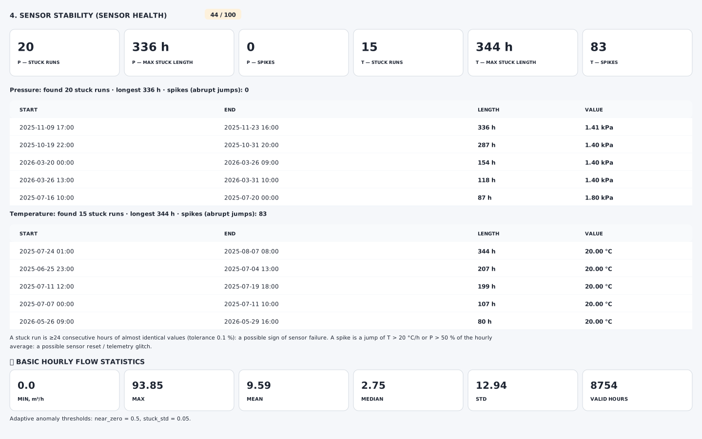
Detailed diagnostics for P and T sensors. Each stuck run gets its start/end/length/value. Long intervals with the same value are almost always a sign of ADC failure / sensor reset / operational flow shutdown — not real physics. Spikes — abrupt jumps ≥ threshold per hour — are conversely a telemetry artefact or sensor reset.
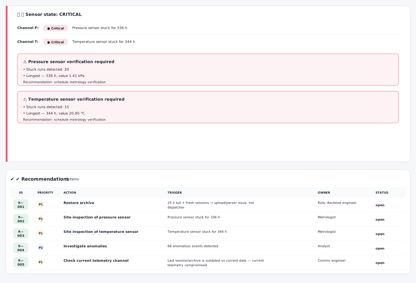
Interpretation and action plan for sensors. “Sensor state: CRITICAL” is a final textual rollup across both channels. Each detected issue is automatically tagged with a recommendation, priority, owner role and a short trigger (what specifically fired).
Stuck sensor
A sensor is considered stuck if the value barely changes for longer than the threshold (24 h):
Sameness tolerance (0.1 %):
Points are considered the same if .
Temperature spike
Pressure spike
Interpretation
| Indicator | Meaning |
|---|---|
| Long T stuck | possible T sensor failure |
| Long P stuck | possible P sensor failure or P_const mode |
| Many P spikes | channel instability or telemetry artifact |
| Many T spikes | sensor error or abrupt technological mode |
Aggregate archive-quality scores
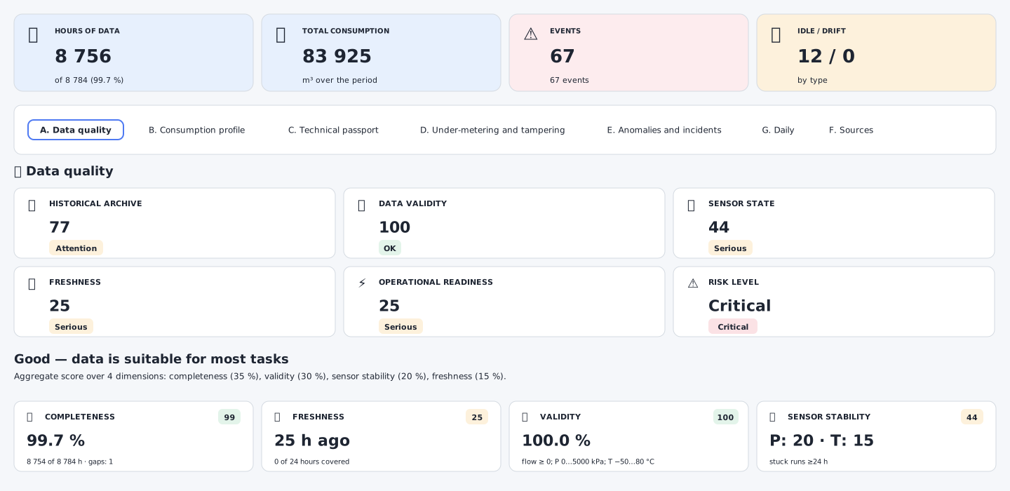
Aggregate quality panel. At the top — the report’s key KPIs (data hours, volume, events, idle/drift). Below — section tabs (data quality, consumption profile, technical passport, under-metering and tampering, anomalies and incidents, daily, sources). On the data-quality tab — 6 sub-indicators 0–100 plus a verbal verdict and composite-score weights.
The report produces 5 orthogonal scores (0–100 each) covering distinct facets of quality:
| Score | About |
|---|---|
score_historical_archive | usability of historical period data |
score_data_validity | correctness of Q/P/T values |
score_sensor_health | sensor state (stuck, spikes) |
score_timeliness | archive and session freshness |
score_operational_readiness | readiness for current monitoring |
Estimated potentially-unobserved volume
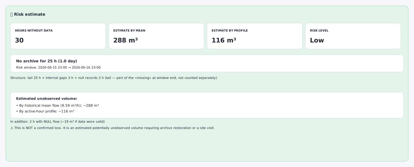
Two different estimates of the same volume. The period mean is conservative (tail backfill under a flat profile), while the active-hour profile better captures diurnal rhythm (work shift / night / weekend). The gap between them is the uncertainty range, not a single point. The risk level depends on gap length and the characteristic mean flow.
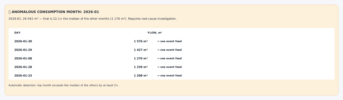
Anomalous consumption month. Monthly anomalies are a separate signal evaluated against the yearly rhythm (heating season vs summer). If a particular month substantially exceeds the median of the others (threshold × 2), it is automatically surfaced at the top with a suggestion to check the event feed, passport and technological causes.
This block estimates how much gas could have passed during hours without valid archive data.
Hours without valid data
Mean-based estimate
Suits objects with relatively uniform consumption.
Profile-based estimate
Typical flow for hour-of-day (median over period):
If the profile for an hour is unreliable, is used.
Estimate range
Both estimates are shown. If close — the daily profile is stable. If they diverge significantly — the object has a pronounced operation mode and caution is required.
Idle node
If a node had virtually no real consumption for the period, the absence of flow is not treated as a risk.
Idle check
Adaptive near-zero threshold:
The node is considered idle when both conditions hold:
Effect
The severity scale becomes softer (max medium instead of critical), and the report states:
The node was effectively offline / seasonally stopped. Absence of consumption is not treated as an under-metering risk.
Q/V reconciliation
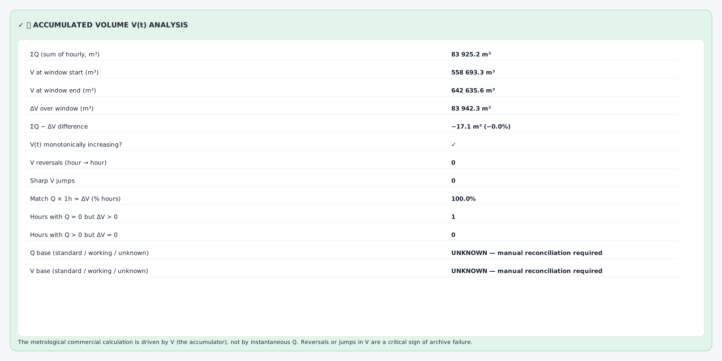
Hourly-flow vs accumulator reconciliation. The metrological commercial calculation is driven by the V increment, not by the sum of instantaneous Q values. A ΣQ ≈ ΔV match ≥ 80 % of hours is the norm for a healthy node. V reversals (hour to hour, ) and sharp V jumps are critical signs of archive failure and almost always require investigation.
The key metrology block. Compares the sum of hourly flows to the cumulative-counter increment.
Base quantities
Mismatch interpretation
| Verdict | |
|---|---|
| ≤ 2 % | good (aligned) |
| 2–5 % | warn (aligned with caveats) |
| > 5 % | bad (mismatch) |
| no V | unavailable |
| Q/V basis unknown | requires passport verification |
Counter monotonicity
The counter must rise or stay flat.
Rollback: → incident V_ROLLBACK.
Sharp jump: → incident V_JUMP.
Per-hour reconciliation
For each hour with both and :
Hour is aligned if . Share of aligned hours:
Limitations of Q/V reconciliation
Even a good numerical match does not equal commercial usability. You need to know:
| Question | Why it matters |
|---|---|
| Q — standard or working volume? | different bases give a bias |
| V — standard or working volume? | need the same basis |
| What is the pulse weight? | required for a full commercial reconciliation |
| Is V monotonic? | rollbacks cast doubt on the archive |
| Are there manual corrections? | they can explain divergence |
If the basis is unknown:
Q/V reconciliation is numerically aligned, but the commercial basis is unconfirmed. Verification of the passport, pulse weight and volume basis is required (see EN 12405-1 §7).
Communications vs archive
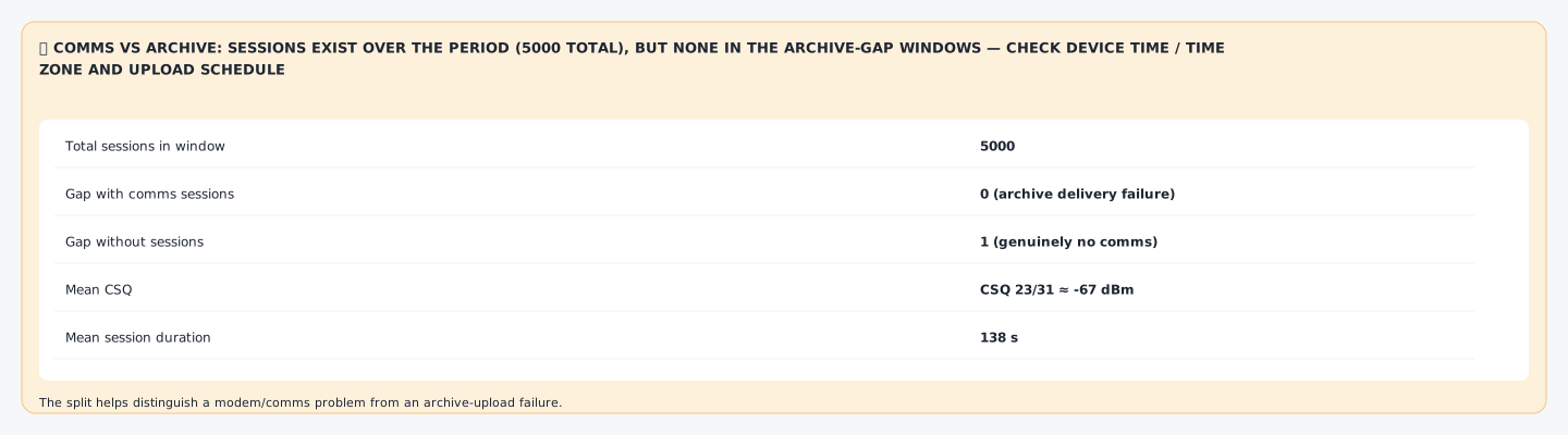
“Comms vs upload” differential diagnostics. If sessions exist in the window but archive does not — the device responds over GSM/CSQ, but the archive is either not written or not parsed by the server. This is not a dispatcher / modem problem — it should be handled by an integration engineer.
Base formulas
Archive delivery
For each gap we check whether sessions occurred in the same time window:
gap_with_sessions— archive gap with sessions present;gap_without_sessions— archive gap and no sessions either.
Differential diagnosis
| Situation | Likely cause |
|---|---|
| no sessions, no archive | modem / SIM / antenna / power |
| sessions OK, archive not updating | hourly archive delivery / parser / import |
| sessions OK but part of archive missing | partial read / page break / backend |
| sessions fresh, archive stale | not a GSM issue, archive-delivery problem |
| session timestamp in the future | clock / timezone mismatch |
Signal quality
If signal quality is reported as CSQ:
Example: CSQ=29 → RSSI ≈ −55 dBm (excellent).
Metrology passport
Required fields with weights
The passport defines 11 fields with weights:
| Field | Weight | Why |
|---|---|---|
| equipment_serial_number | 1.0 | identification |
| equipment_type_id | 1.0 | model/type |
| installation_date | 0.8 | operational context |
| verification_date | 1.5 | legal validity (OIML R 137 cl. 3) |
| next_verification_date | 1.0 | term control |
| flow_range (Qmin/Qmax) | 1.5 | range under EN 12405-1 |
| meter_serial_number | 1.0 | on-site identification |
| meter_type | 1.0 | metrology binding |
| firmware_version | 0.5 | compatibility and known bugs |
| p_const | 0.5 | substituted pressure |
| pulse_weight | 0.8 | for Q/V reconciliation |
Completeness formula
Interpretation
| Completeness | Status |
|---|---|
| ≥ 80 % | COMPLETE |
| 50–80 % | PARTIAL |
| 20–50 % | INCOMPLETE |
| < 20 % | CRITICAL_INCOMPLETE |
If the passport is incomplete the commercial verdict must include a caveat:
Metrology passport incomplete. Commercial verdict requires manual reconciliation and reference to OIML R 137 / EN 12405-1.
Suspicious under-metering patterns
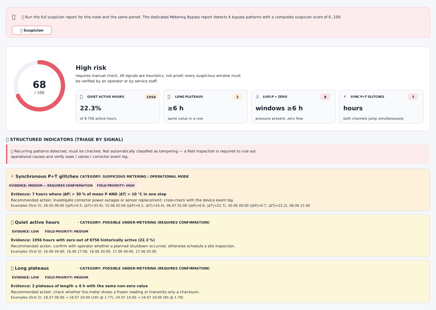
Signal triage. Each signal is classified into a category, has an evidence level (low / medium / high), a field priority, formal evidence and a recommended action. This is not a verdict on the node — it is a list of windows that need manual checking by an operator or by service staff.
These are heuristics, not proofs.
Near-zero threshold
Zero flow during active hours
An hour is suspiciously quiet if AND falls into the object’s typical active interval.
Live-P + zero (Q≈0 with live P)
May be:
- shutdown / closed downstream valve / seasonal stop;
- P_const mode or sensor failure;
- pulse-input error;
- possible tampering — but not proven.
Break-recovery
Pattern: normal Q → Q≈0 → normal Q. Sharp mode change but not a violation proof. Possible explanations: planned shutdown / object stoppage / valve closure / channel failure / manual intervention / archive-delivery error.
Confirmed tampering
A statistical pattern alone cannot confirm tampering. You need hard evidence:
- cabinet opening (cover_open in device events);
- magnetic interference;
- parameter changes (parameter_change);
- unauthorised P_const modification;
- archive reset;
- confirmed pulse-input manipulation;
- site-visit acceptance act;
- photos / seals / on-site readings.
Correct verdict format:
Confirmed tampering: NOT DETECTED
Suspicious patterns:  PRESENT
Legal readiness:      NOT READY
Commercial Metering Verdict
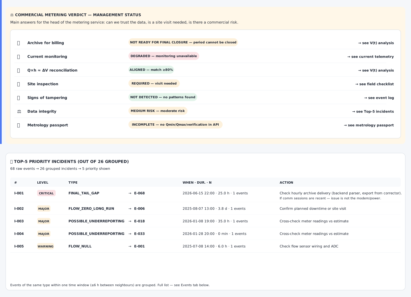
Management status. The 7 rows close 7 different manager-level questions: can the period be closed (billing), is the node working now (monitoring), do archive and accumulator match (Q×h vs ΔV), is a site visit needed, are suspicious patterns present, how integral is the data, are all passport parameters present. Each row is clickable and points to the evidence block of the report.
The headline verdict for the metering-service manager.
Billing-archive rules
Ready:
- Coverage ≥ 98 %
- Tail gap ≤ 2 h
- Q/V aligned (
good) - V monotonic
- Passport COMPLETE
- No critical sensor issues
Ready with caveats:
- Coverage 95–98 %
- Tail gap 2–24 h
- Q/V aligned with caveats (
warn) - Passport PARTIAL
- No critical blocker
Not ready for final closure:
- Tail gap > 24 h OR
- Q/V not classified OR
- V rollback present OR
- Passport incomplete in commercial fields OR
- Critical sensor issue
Not usable:
- Coverage critically low OR
- Archive corrupted OR
- V has major rollback/spikes OR
- Q/V completely inconsistent OR
- Key channel unavailable
Current monitoring — assessed separately
| Condition | Status |
|---|---|
| archive and session fresh | usable |
| archive lagging but sessions present | degraded / delivery issue |
| archive and sessions stale | critical / communication issue |
| timestamp invalid | unreliable |
Field inspection
A visit is required if at least one of:
- tail gap not restored;
- Q/V not classified;
- counter rollback present;
- passport critically incomplete;
- P or T sensor stuck;
- suspicious under-metering patterns;
- event journal unavailable while strong anomalies exist;
- current telemetry critically degraded.
Incidents
An incident is a grouped issue, not every raw record.
Types
| Type | Meaning |
|---|---|
FINAL_TAIL_GAP | no data at the end of the period |
COMMUNICATION_GAP | comms outage |
ARCHIVE_DELIVERY_GAP | sessions present, archive not delivered |
Q_V_MISMATCH | Q and V don’t add up |
V_ROLLBACK | counter rolled back |
P_SENSOR_STUCK | pressure stuck |
T_SENSOR_STUCK | temperature stuck |
PASSPORT_INCOMPLETE | passport fields missing |
TAMPERING_CANDIDATE | suspicious pattern, not proof |
Grouping principle
raw events → grouped incidents → top priority incidentsExample: 301 raw → 15 grouped → Top-5 for action. The operator must not be shown 301 identical events as 301 separate problems.
Action plan
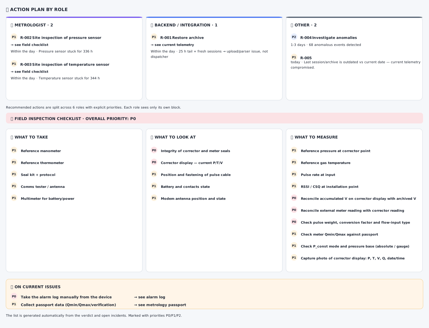
Actions with P0/P1/P2 priorities. Every action carries an owner role, a deadline (today / within the day / 1–3 days) and the cause that put it on the list. The field checklist is built automatically from the verdict and open incidents: what to take, what to look at, what to measure — labelled P0/P1 for on-site prioritisation.
Each recommendation is tied to a cause.
| Field | Description |
|---|---|
| ID | recommendation number |
| Priority | P0 / P1 / P2 / P3 |
| Action | what to do |
| Role | who is responsible |
| Deadline | when to complete |
| Cause | why this action arose |
| Status | open / assigned / done / verified |
Rule examples
| Condition | Action |
|---|---|
| tail > 24h, sessions fresh | backend: restore hourly-archive delivery |
| tail > 24h, no sessions | comms: check modem/SIM/power |
| T stuck ≥ 24h | metrologist: verify T sensor (OIML R 137) |
| P stuck ≥ 24h | metrologist: verify P sensor or P_const setting |
| Q/V mismatch | metrologist + billing: reconcile V, Q, pulse weight (EN 12405-1 §7) |
| passport incomplete | admin / metrologist: fill the passport |
| suspicious patterns | field crew: check seals, pulse input, valves |
Field checklist
What to bring
reference manometer • reference thermometer • multimeter • signal/antenna tester • seal kit • inspection protocol • access to archive and passport • photo capture.
What to check
corrector and meter seals • pulse cable • P, T sensors • modem, antenna, power, battery • shutoff valves • possible bypass • passport vs actual equipment.
What to measure
reference P, T • current Q • cumulative V • external meter readings • CSQ/RSSI • supply voltage • input pulses • corrector date/time • P_const • Qmin/Qmax • pulse weight.
What to photograph
corrector display (P/T/Q/V) • date/time on device • serial numbers • seals • pulse cable • sensors • modem and antenna • general view • valve positions.
Source by behavioural profile
The specific API archive and field are selected automatically by device behaviour. Three families:
Continuous hourly archive
The device writes a record exactly once per hour. Source priority:
- direct “flow per hour” field (if the device computes it);
- Δ of cumulative standard volume;
- Δ of cumulative working volume.
Acceptable gap — exactly 1 hour.
Session-based upload with current-state archive
The device writes records when it connects, not strictly hourly. The primary source is instantaneous flow (device-computed); fallback is Δ of cumulative volume normalised:
Acceptable gap — up to 6 hours; if the point is considered invalid (likely data loss, not counter discharge).
Pure-telemetry blocks
The device transmits only comms/state, does not measure gas — the report shows N/A with “this device has no metering point”.
Sparse-fallback
If the primary archive yields < 50 % of expected points, the secondary sessions archive is tried automatically (as is, without an hourly grid) and computation proceeds from it.
Methodology limitations
Archive
If the hourly archive is incomplete, all estimates for missing hours are approximate.
Q/V
Q/V reconciliation is meaningful only when Q and V:
- share a single volume basis (standard or working);
- have a correct pulse weight;
- belong to the same metering source;
- are time-synchronised.
See OIML R 137 for the verification procedure and EN 12405-1 §7 for conversion basis.
Passport
Without Qmin/Qmax, verification date, P_const or pulse weight, the commercial verdict must carry a caveat.
Suspicious patterns
Under-metering patterns are not proof of tampering. They only set the priority for inspection.
AI commentary
AI commentary takes no part in the legal verdict and does not replace formal rules. It only helps explain the situation in plain language.
How to read the report
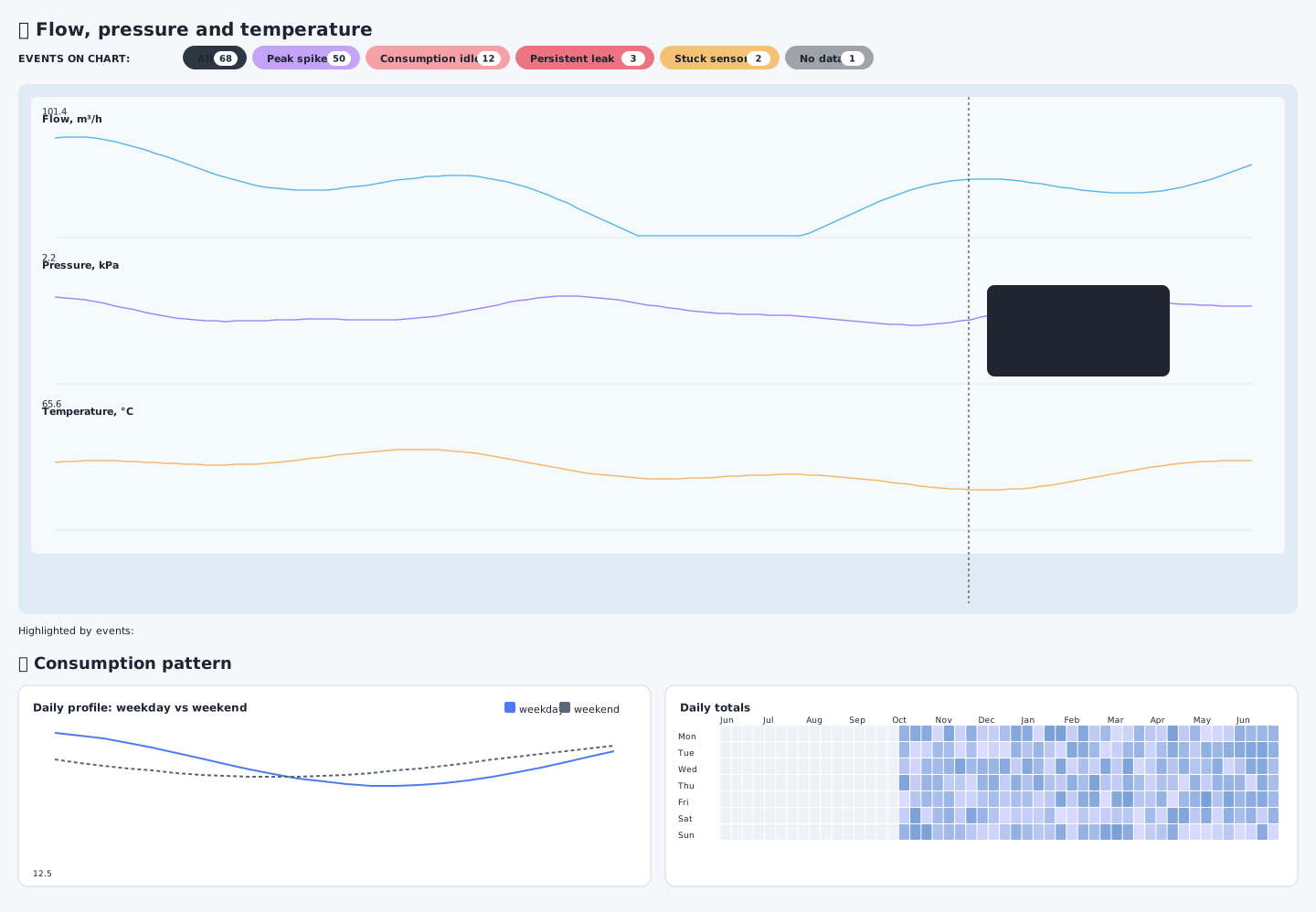
Q/P/T visualisation and behavioural profiles. On the main chart, events are highlighted as semi-transparent vertical bands by type (spike / idle / leak / stuck sensor / no data) — any type can be shown/hidden by clicking its chip. Rolling 7 / 30-day means provide seasonal smoothing. The consumption pattern is a double breakdown: daily profile (hour of day) split by weekday/weekend, and a calendar heatmap “day-of-week × month” showing work-shift stability.
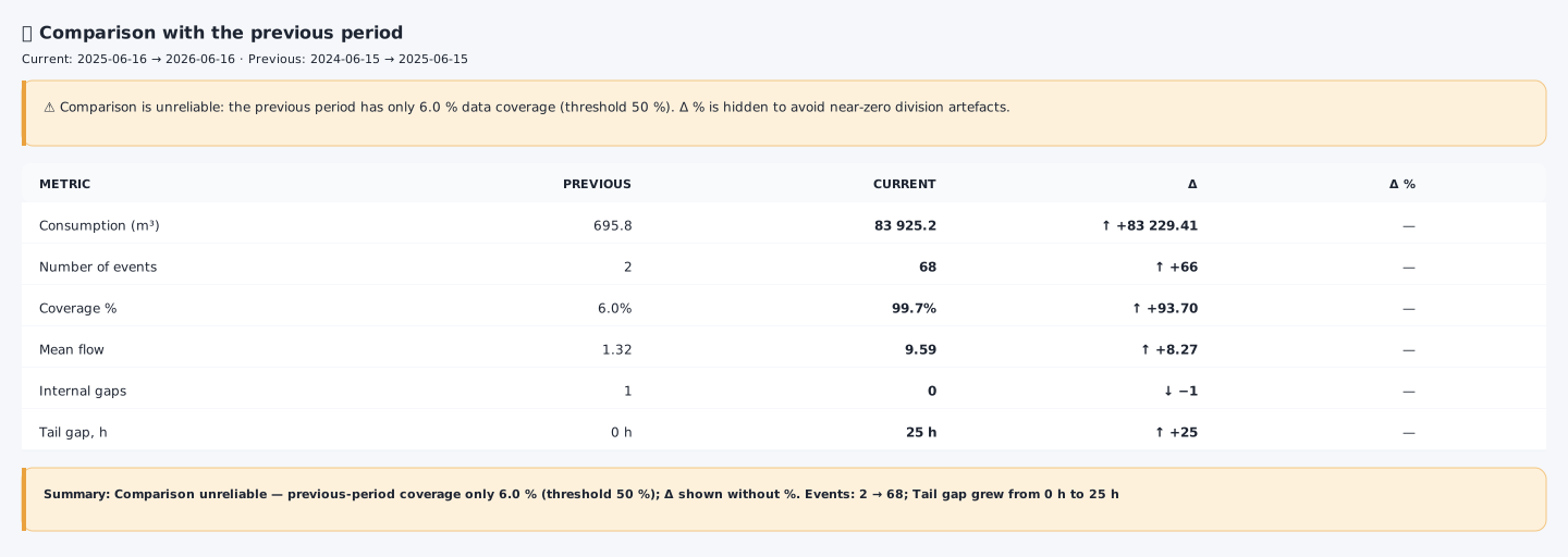
Period-over-period comparison. A year-over-year delta carries two traps: (1) change of previous-period coverage (if it was 6 %, a “33×” event growth is a division artefact, not reality) and (2) no length normalisation. So with coverage < 50 % the comparison masks Δ % and shows absolute deltas only, to avoid leading the operator to false conclusions.
- Start with the Commercial Metering Verdict.
- See whether the period is ready for billing.
- Separately check current monitoring.
- Move on to Top-5 incidents.
- If there is a tail — go to “comms vs archive”.
- If there is a Q/V discrepancy — go to the accumulated-volume analysis.
- If P/T sensors are stuck — go to sensor stability.
- If the passport is incomplete — do not issue a hard commercial verdict.
- If suspicious patterns exist — plan a check, but do not issue a legal verdict.
- Execute the action plan by role.
Minimum criteria for a complete report
A report is considered complete if it contains:
-
analysis period • • received records • valid records • NULL records • internal gaps • tail gap • coverage • freshness • Q/P/T validity • sensor health • unobserved-volume estimate • Q/V reconciliation • V monotonicity • comms vs archive • passport completeness • Top-5 incidents • action plan by role • field checklist;
-
three mandatory disclaimers:
- on under-metering (this is a blind-spot estimate, not a loss figure);
- on tampering suspicion (patterns ≠ proof);
- on AI commentary (not a legal verdict).
Run parameters
| Parameter | Description |
|---|---|
| Metering node # | the metering node to analyse |
| Period from | start of the analysis window (default: one year back) |
| Period to | end of the analysis window (default: yesterday) |
| Extended analysis | additionally loads the comms-sessions archive and the corrector abnormal-events archive. Enables the Data Source Readiness, Communication Health and Device Abnormal Log blocks and fills the Root Cause Matrix with confidence and root cause per event. Adds 5–15 seconds to report build time. |
Related topics
Was this page helpful?
Thanks for your feedback!