Suspicious Nodes
Ranks fleet metering nodes by the probability of under-metering using six independent forensic signals combined as probabilities, not a sum.
The Suspicious Nodes report performs a fleet-wide analysis of gas metering nodes and ranks the points that require priority verification for possible under-metering, measurement-channel substitution, incorrect settings, abnormally low consumption, or device events related to physical access and parameter changes.
It draws on the normative framework for gas metering — ISO 5167 (orifice plates), ISO 6976 (calorific value), EN 12405-1 (electronic gas-volume conversion), OIML R 137 (gas meters), OIML R 140 (measuring systems for gaseous fuel) and EN 1359 (diaphragm meters).
This is not an operational report about communication, battery or archive quality — those tasks belong to a separate operational report on problem nodes. This report focuses specifically on forensic signals: behavioural, metrological, comparative and event-based indicators that may suggest the need for a metering-service check.
The report’s main task is not to prove a violation, but to set verification priorities correctly:
- which nodes to check first;
- where there are several independent signals;
- where consumption is abnormally low compared with similar nodes;
- where there is a combination of zero flow, live pressure and an incomplete passport;
- where the standard and working volume diverge more than physical P/T-correction can explain;
- where the expected seasonal growth in consumption is absent;
- where there were device events related to physical access or reading substitution;
- where it is worth opening the detailed report on a specific node.

The report header shows the fleet size, how many nodes entered deep analysis, the covered period and the generation time. These three numbers are distinct entities: the total fleet, the analysed candidates, and the TOP-N rows in the table.
Where this report fits
The Suspicious Nodes report sits between fleet-wide operational monitoring and the detailed forensic breakdown of a single node.
| Report | Main question | Scale |
|---|---|---|
| Operational problem nodes | where there are communication, battery, passport, archive issues | fleet |
| Suspicious Nodes | where there are forensic signals of possible under-metering | fleet |
| Metering Bypass (node) | why a specific node looks suspicious | one node |
| Consumption Analytics | whether a specific node’s data is fit for metering and analysis | one node |
A node can be operationally bad but not suspicious from the under-metering point of view, and vice versa: a node can be stably online with a good archive yet consume suspiciously little relative to its cohort.
Who the report is for
| Role | How they use the report |
|---|---|
| Head of metering service | chooses priorities for checks and field visits |
| Metrologist | analyses the causes of suspicion and the need to verify the passport |
| Dispatcher | dispatches tasks for high-priority nodes |
| Field team | receives the node list and a link to the detailed breakdown |
| Analyst | checks cohorts, seasonality, anomalies and events |
| Billing analyst | estimates the potential commercial scale of the risk |
| Control service | separates weak signals from cases requiring investigation |
| Legal | uses it as grounds for launching an investigation (not as proof) |
What the report does not do
The report must not:
- prove the fact of metering bypass;
- automatically accuse a consumer;
- replace a field check;
- treat the loss estimate as confirmed damage;
- interpret low consumption as a violation without comparison with the object’s regime;
- treat the absence of data as a zero signal;
- mix operational issues with forensic signals;
- treat an unavailable indicator as equal to zero;
- make a legal conclusion based on the AI summary;
- replace the detailed report for a specific node.
Key terms
| Term | Meaning |
|---|---|
| Node | a gas metering point whose telemetry is analysed |
| Fleet | the set of all nodes of a company |
| Candidate | a node that passed the pre-selection for deep analysis |
| Cohort | a group of similar nodes for consumption comparison |
| Percentile | the node’s position by flow among similar nodes |
| Subscore | a partial score for one forensic signal from 0 to 100 |
| Composite score | the final suspicion score |
| Ceiling | the maximum contribution of a signal to the final probability |
| Direct signal | a direct behavioural forensic signal based on Q/P/T |
| Peer anomaly | flow anomaly relative to similar nodes |
| Passport bypass | the signature “empty passport + near-zero flow + live pressure” |
| Divergence | divergence between standard and working volume beyond physical explanation |
| Seasonal anomaly | absence of the expected seasonal growth |
| Event recency | freshness of device events related to access or substitution |
| Cluster flag | indicator that one organisation has several suspicious nodes |
| Estimated losses | commercial priority: score x consumption, not confirmed damage |
General report logic
The report is built as a fleet-wide suspicion filter.
All fleet nodes
→ pre-selection of live forensic candidates
→ deep analysis of the hourly archive and events
→ calculation of 6 independent subscores
→ comparison of nodes with the cohort
→ composite score calculation
→ cluster correction by organisation
→ TOP-N ranking
→ output of the level distribution
→ list of actions and links to detailed reports
The key principle: the report looks not just for “bad” nodes, but for nodes with signs of possible under-metering in the presence of data. A fully dead node that has not transmitted data for a long time is an operational problem, but not necessarily a good forensic candidate.
Input data
Minimum required data
| Data | What it is needed for |
|---|---|
| Node list | to form the analysis fleet |
| Device type | to build cohorts |
| Organisation | to compare within similar groups |
| Consumption over the period | for ranking and scale estimation |
| Hourly archive Q/P/T/V | for behavioural signals |
| Analysis period | for seasonality and events |
Additional data
| Data | What it is needed for |
|---|---|
| Communication sessions | for the “archive gap with successful sessions” indicator |
| Device passport | for the passport-bypass indicator |
| Corrector settings | for P_const, pulse weight, correction parameters |
| Device event log | for physical access, substitution, reset, parameter change |
| Previous data on similar nodes | for the peer baseline |
| Seasonal window data | to check the winter/summer profile |
Minimum period for reliable scoring
A period shorter than 30 days automatically makes the seasonal signal unavailable. The recommended minimum is 90 days. A full seasonal analysis is only possible on a period of at least 6 months covering both seasons.
Run parameters
| Parameter | Meaning |
|---|---|
| Period from / Period to | the evaluation window (defaults to the last 90 days) |
| How many nodes in top | size of the final TOP-N table |
| How many nodes to deep-analyze | number of candidates retained after pre-selection |
| Resource company | restrict the analysis to one organisation, or use the whole fleet |
| Organization clustering | add +10 to nodes of organisations with two or more suspicious nodes |
| AI fleet summary | optional human-language commentary that does not affect scores |
Report scope
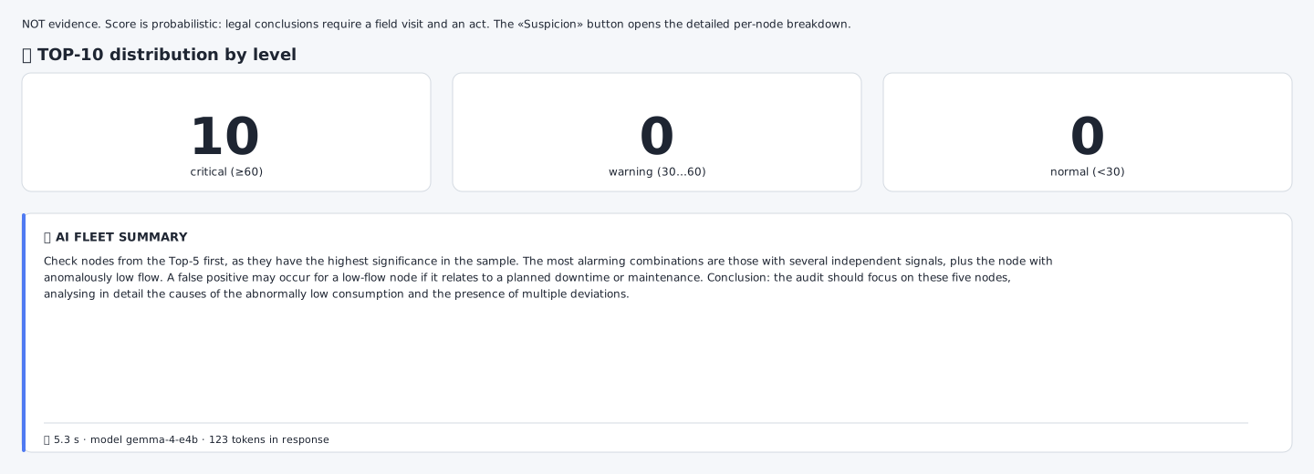
Right under the report header are three distribution cards and an AI-comment block. They are read together: the distribution gives a quick answer to “how many nodes are critical”, and the AI summary explains why exactly these nodes reached the top and what to pay attention to.
The top block shows:
| Indicator | Value |
|---|---|
| Total nodes in the fleet | size of the whole fleet |
| Analysed | how many nodes entered the deep analysis |
| TOP-N | how many nodes are shown in the final table |
| Period | evaluation window |
| Data retrieval errors | how many candidates could not be fully processed |
| Level distribution | critical / warning / normal |
It is important to distinguish:
Total fleet nodes ≠ number of deeply analysed nodes ≠ number of rows in TOP-N.For example, the fleet may contain hundreds of nodes, deep analysis may be performed on a set of candidates, and the report shows only the TOP-N.
Level distribution
| Composite | Level | Card colour |
|---|---|---|
| ≥ 60 | critical | red |
| 30–60 | warning | orange |
| < 30 | normal | green |
A high concentration in red is not a reason to panic, but a signal to carefully check the top: possibly the methodology gave a strong response to a specific operating regime rather than to real interference.
Pre-selection of forensic candidates
Before deep analysis the report prioritises nodes for which it is at all possible to look for forensic patterns.
Why live nodes are needed
For the suspicion report, nodes with data are important. If a node is fully dead, it does not give a sufficient picture of Q/P/T, and it should be checked in the operational communication report, not in the forensic ranking.
A typical principle:
a bypasser does not necessarily disable telemetry completely;
they may disguise themselves as a "low consumer".
The pre-selection therefore considers the freshness of the last session, the presence of non-zero volume, the device status, and the presence of data in the archive.
Pre-selection scoring
The preliminary score can be described as:
where:
| Component | Logic |
|---|---|
AliveScore | higher if the node was recently online |
VolumeScore | higher if there is registered volume |
StatusScore | higher if the node is in working or sealed state |
The preliminary score is not the final suspicion score. It only selects candidates for deeper analysis.
Six suspicion signals
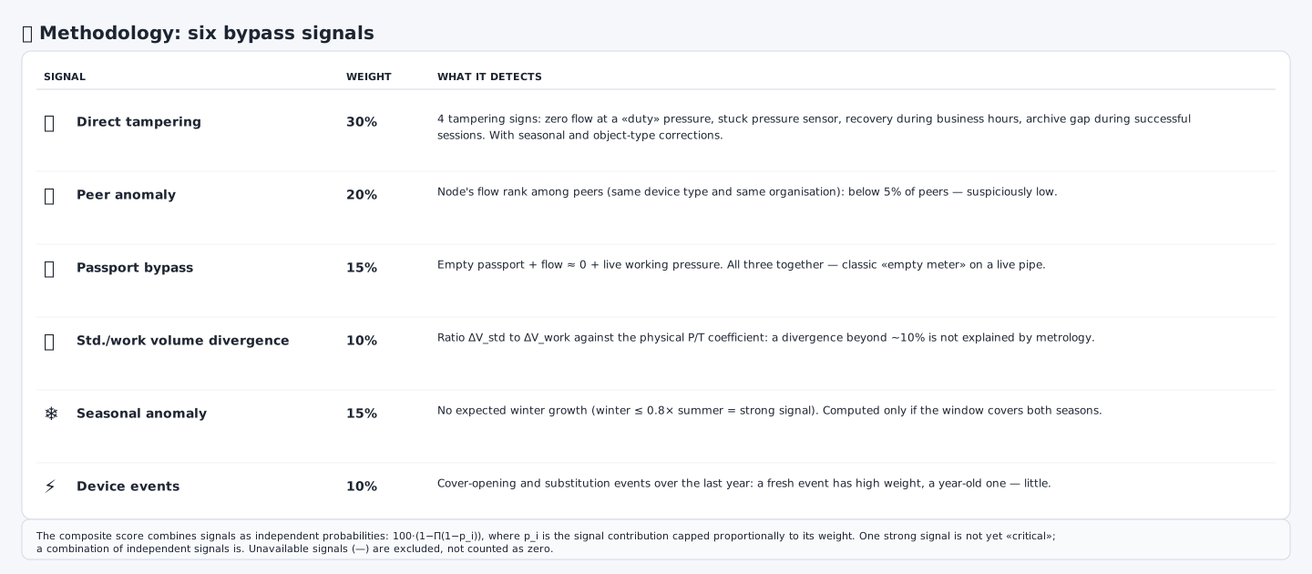
All six detectors are shown with their description, documentation weight and probabilistic-contribution ceiling. The final score is not a sum but a probabilistic composition. One strong signal alone is not yet “critical”; a combination of independent signals is. Unavailable signals are excluded, not counted as zero.
| # | Signal | Documentation weight | Maximum probabilistic contribution |
|---|---|---|---|
| 1 | Direct tampering | 30% | 0.85 |
| 2 | Anomaly relative to cohort (peer anomaly) | 20% | 0.57 |
| 3 | “Dummy” signature (passport bypass) | 15% | 0.43 |
| 4 | Standard vs. working volume divergence | 10% | 0.28 |
| 5 | Seasonal anomaly | 15% | 0.43 |
| 6 | Device events with recency | 10% | 0.28 |
Percentage weights are used for documentation and explanation. The final formula uses not a linear sum but probabilistic ceilings (see the probabilistic model).
Signal 1 — direct tampering
This signal reuses behavioural forensic patterns from the hourly archive. It shows whether the node has signs of possible measurement-channel substitution or suspicious zero flow with a working pipe.
Typical indicators that may enter the direct signal:
- zero flow at working or substituted pressure;
- frozen pressure channel;
- recovery of flow and pressure after a zero window;
- archive gap with successful communication sessions;
- contextual corrections for season, object type and consumption regime.
The detailed methodology of direct patterns is described in the Metering Bypass (node) report, which defines nine formal detectors with thresholds.
The direct subscore has the range:
where:
0— direct behavioural signs not found;30–60— weak or medium signs present;60–100— strong or repeated signs present.
The direct signal is not proof. It means: open the detailed report on the node and inspect the event windows.
Signal 2 — anomaly relative to cohort
Comparison with the cohort answers the question: does the node consume suspiciously little compared with similar nodes? Similar nodes are those with the same device type and the same organisation or another specified grouping.
For comparison the rate is used:
where Consumption_i is the total consumption of the node over the period and Hours_i is the number of hours of data.
The percentile shows the node’s position in the cohort by flow:
A low percentile means the node consumes less than most similar nodes. For example, Percentile = 5% means the node consumes less than about 95% of similar nodes.
Base score by percentile
| Percentile | Base score |
|---|---|
| < 3% | 100 |
| < 5% | 85 |
| < 10% | 60 |
| < 25% | 30 |
| ≥ 25% | 0 |
Adjustment for distance from the median
A low percentile alone does not always mean suspicion: in any cohort someone will be last. The score is therefore scaled by the ratio to the cohort median.
| Ratio to median | Factor |
|---|---|
| ≤ 0.33 | 1.0 |
| 0.33–0.50 | 0.6 |
| 0.50–0.70 | 0.3 |
| > 0.70 | 0.0 |
Final peer score:
Interpretation
| Peer score | Meaning |
|---|---|
| 0 | consumption does not look suspiciously low |
| 30 | a weak anomaly is present |
| 60 | the node is noticeably below the cohort |
| 85–100 | the node is sharply below similar nodes |
Signal 3 — “dummy” signature (passport bypass)
The signal looks for a combination of three factors:
- the device passport is almost empty;
- flow is almost zero for most of the period;
- pressure at the same time is working and live.
Such a combination may look like a “dummy on an active pipe”: there is gas in the pipe and pressure is present, but flow is barely registered, and passport data is insufficient for verification.
Zero-flow share
Let:
Then:
Zero-flow condition:
Live working pressure
The median pressure is computed:
and the standard deviation of pressure:
Pressure is considered working and live if:
and:
That is, the pressure is above atmospheric level and does not look fully frozen.
Empty passport
The passport is considered empty or critically incomplete if a significant part of the mandatory fields is missing:
- verification date;
Qmin/Qmax;- meter type;
- meter serial number;
P_const;- pulse weight;
- pressure type;
- firmware version.
Score formula
Let:
A = PassportEmpty
B = ZeroShare ≥ 0.60
C = P_median > 103 and σP > 0.05
The number of satisfied conditions:
Score:
| Number of conditions | Score |
|---|---|
| 3 | 100 |
| 2 | 50 |
| 0–1 | 0 |
This signal does not mean proven bypass. It shows that the node requires documentary and field verification.
Signal 4 — standard vs. working volume divergence
Many correctors transmit both a working volume and a converted / standard volume after P/T correction. Normally the ratio of the standard-volume increment to the working-volume increment should roughly correspond to the physical P/T correction coefficient.
Actual volume ratio
Let:
be the increment of standard or corrected volume, and:
the increment of working volume.
Then the actual ratio:
Expected P/T coefficient
The approximation used is:
where:
- ;
- , i.e. 20°C;
- — mean pressure;
- — mean temperature in °C.
Relative divergence
Score
Up to 10% divergence is considered an acceptable zone.
| Divergence | Score |
|---|---|
| ≤ 10% | 0 |
| 20% | 25 |
| 30% | 50 |
| 50% and above | 100 |
When the signal is unavailable
The signal is considered unavailable if:
- there is no standard-volume channel;
- there is no working-volume channel;
- there are too few valid hours;
- volumes are not monotonic;
- the sum of working volume equals zero;
- there is no P/T data for the expected coefficient.
Signal 5 — seasonal anomaly
For many gas consumers a winter increase in flow is expected. If the period contains both winter and summer months but winter flow does not grow or even falls, this may be a signal of under-metering in the peak consumption season.
Winter months are December, January and February. Summer months are May, June, July, August and September.
Availability condition
The seasonal signal is counted only if there is sufficient data in both seasons:
and:
If there is less data, the signal is considered unavailable.
Average flow by season
Seasonal ratio
Score
| Condition | Score |
|---|---|
| 100 | |
| 60 | |
| 30 | |
| 0 |
For industrial consumers without heating load, seasonal growth may be absent. The seasonal anomaly must therefore be interpreted with the object type in mind.
Signal 6 — device events with recency
Device events can be more significant than statistical anomalies. Especially important are events of physical access, cover opening, parameter changes, reading substitution, reset, time changes, and events affecting the measurement channel.
Event base score
| Event class | Base score |
|---|---|
physical | 100 |
substitution | 70 |
Event age and decay
Event age:
Decay coefficient:
A fresh event has full weight; an old event gradually loses significance; the minimum residual weight is 20%.
Event score
Final recency score
If there are several events, the maximum score is taken:
If the log is available but there are no events, . If the log is unavailable, the signal is unavailable and is excluded from the final formula.
Unavailable signal ≠ zero signal
This is one of the key rules of the report. If a signal cannot be calculated due to lack of data, it receives the status — (unavailable), not 0.
Reasons for unavailability:
- no required archive channel;
- not enough hours;
- no event log;
- no seasonal coverage;
- no cohort data;
- no working or standard volume;
- no passport.
In the final formula, unavailable signals are excluded from the product, neither decreasing nor increasing the score.
Probabilistic model of the final score
If all six signals were simply summed with weights, one strong signal could look like full proven risk, and many weak signals could mechanically create false criticality. A multiplicative model of independent probabilistic contributions is used instead.
Ceiling for each signal
Each signal has a maximum contribution:
| Signal | Ceiling |
|---|---|
direct | 0.85 |
peer | 0.57 |
bypass | 0.43 |
divergence | 0.28 |
seasonal | 0.43 |
recency | 0.28 |
Probabilistic contribution of a signal
Let S_i be the signal subscore from 0 to 100 and C_i the signal ceiling. Then the contribution:
Probability of absence of all signals
Final score
that is:
Example
Suppose there are three signals:
| Signal | Subscore | Ceiling | |
|---|---|---|---|
direct | 90 | 0.85 | 0.765 |
peer | 50 | 0.57 | 0.285 |
seasonal | 30 | 0.43 | 0.129 |
Then:
Model interpretation
- one strong signal can give a high score, but not a full 100;
- a combination of independent signals sharply raises the priority;
- weak signals do not add up linearly;
- unavailable signals do not penalise the node;
- the final score is the verification priority, not proof.
Cluster correction by organisation
If one organisation has several suspicious nodes, this raises the verification priority. Such cases may indicate a systemic operating regime, settings, maintenance or potentially coordinated actions.
If one organisation has:
and each of these nodes has:
then each node receives a cluster correction:
The cluster correction is not proof. It only raises the verification priority, because several nodes of one organisation require joint analysis.
Level distribution
The final score is translated into a level.
| Composite | Level |
|---|---|
| ≥ 60 | critical |
| 30–60 | warning |
| < 30 | normal |
A threshold of 60 means that the node has a strong signal or a combination of several independent signals. This does not mean proof — it means the node must enter the priority verification list.
TOP-N table
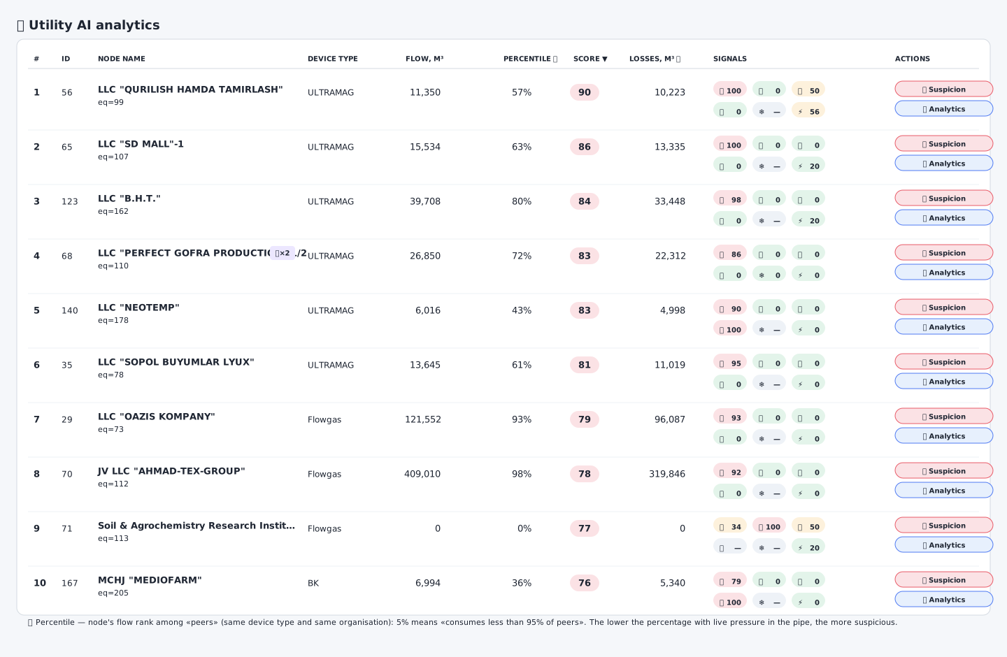
Nodes are sorted by the final suspicion score. Each row contains six badge indicators for the signals, which lets you see at a glance why the node entered the top. Numbers in badges are 0…100 or —; the — sign means “could not be computed”.
Main columns
| Column | Meaning |
|---|---|
Rank (#) | place in the ranking |
ID | node identifier |
| Node name | object name |
| Device type | corrector / telemetry type |
| Consumption, m³ | total consumption over the period |
| Percentile | flow rank among similar nodes |
| Score | composite score |
| Losses, m³ | commercial priority, not confirmed damage |
| Signals | subscore values (6 badges) |
| Actions | links to the detailed report and analytics |
How to read the signals
In the table each signal is shown as a separate indicator:
0— signal computed and did not fire;—— signal unavailable;>0— signal fired with the indicated strength.
It is very important that — is not equal to 0.
Action links
| Link | What it opens |
|---|---|
| Suspicion | the Metering Bypass (node) report |
| Analytics | the Consumption Analytics report |
The “Suspicion” link is the main transition point for the field team and the investigator: the full forensic methodology is disclosed in that detailed report.
The “losses, m³” score
The “losses, m³” column is not a confirmed volume of theft. It is a commercial priority that combines the scale of node consumption and the final suspicion score:
where Consumption is the total node consumption over the period and Composite is the final suspicion score.
For example, if Consumption = 100000 m³ and Composite = 80, then EstimatedLossPriority = 80000 m³. This does not mean that 80,000 m³ have been lost. It means the node has a large commercial verification scale: large consumption x high score.
Analytics and conclusions

The summary below the table presents key numbers across the fleet: how many nodes have several independent signals (the most worrying combination), how many have a peer anomaly, and how many are in clusters. The last bullet is a mandatory reminder of the report’s legal status.
The analytics block shows how many nodes were analysed, how many reached the critical level, how many are in the warning zone, how many have two or more independent signals, how many consume abnormally little relative to the cohort, how many are in organisation clusters, and a reminder that the final score is not proof.
Nodes with several independent signals
A node is considered especially important for verification if:
where a strong subscore is:
Such nodes are often more important than nodes with a single isolated signal — the independence of the suspicion sources sharply raises trust in the ranking.
Nodes with peer anomaly
The number of nodes with abnormally low flow is counted by the condition:
Organisation clusters
The number of cluster nodes is counted as the number of rows with a cluster flag.
Device events timeline

Chip buttons open the timeline by the device types observed in the TOP-N. The goal is to see mass synchronous events: “vertical columns” on the time axis indicate coordinated actions in one district or mass maintenance.
The timeline displays events over time for the device types appearing in the TOP-N. It helps to see mass events on a single day or hour, find vertical columns of events, tell an individual case from a systemic one, and understand whether there was mass maintenance, an update or a failure.
| Timeline view | Possible explanation |
|---|---|
| isolated events | individual node problem |
| several events for one organisation | cluster check |
| many events for one device type | systemic model feature |
| vertical column in time | mass action, update, failure, maintenance |
| events before a score increase | possible link with settings or interference |
The AI summary
The AI summary is generated only as a human-language explanation of already-calculated results. It can briefly explain which nodes to check first, indicate which combinations of signals are most worrying, remind of possible false positives, and formulate a general conclusion for the manager.
The AI summary cannot change the composite score, change the critical/warning/normal level, confirm a violation, replace formulas, replace a field visit, replace the detailed node report, or create evidence.
False positives
Low consumption
Low consumption can be normal if the object was idle, there was a seasonal shutdown, the object did not work according to the contractual schedule, the production profile changed, the node serves a backup line, or the cohort was chosen too broadly.
Absence of winter growth
The absence of winter growth can be normal for technological consumers without heating, summer-only production, objects with constant load, objects using gas not for heating, or premises with a non-standard regime.
Device events
A device event can be routine if maintenance was carried out, there was verification, the battery was changed, the time was adjusted according to the regulations, the archive was read, or planned works were performed.
Peer anomaly
A node may be at the bottom of the cohort simply because the cohort is small, the object differs in capacity, devices of the same type are on different loads, the organisation has different kinds of objects, or the period contains downtime.
Hard gates and limitations
- No data — no forensic conclusion. If there is no hourly archive, forensic signals must be unavailable. No data does not mean no suspicion; it means it is impossible to evaluate.
- Unavailable signals are excluded. An unavailable signal does not participate in the product.
- A fleet report cannot confirm interference. A fleet report does not have sufficient detail for an act. It only opens the path to the detailed node report.
- “Losses” cannot be used as a damage amount.
EstimatedLossPriorityis a ranking of the commercial verification scale. - Different object types cannot be compared without a cohort. Flow comparison must be performed only within similar groups.
How to read the report
- Look at the distribution. If many nodes are in critical, determine whether these are real independent signals or an over-sensitive methodology.
- Open the top candidates. The highest-ranked nodes are the priority candidates for verification.
- Look at the signals, not only the score. Two nodes with the same score may have different causes — a direct forensic pattern, a peer anomaly, seasonality or device events.
- Check the commercial scale. Large consumption x high score is more important than small consumption x high score.
- Open the detailed report. The “Suspicion” link leads to the detailed report on the specific node.
- Check false causes. Before a field visit, check seasonality, object downtime, maintenance, consumer type, cohort correctness, the passport and device events.
The correct final conclusion
The correct conclusion from the report sounds like this:
The report identifies nodes with an elevated probability of under-metering
or metering bypass on the basis of independent mathematical and event signals.
The final score is used for prioritising verifications.
For a legal conclusion a detailed node breakdown, a field visit, seal check,
control measurement and documentary confirmation of device parameters are required.
An incorrect conclusion would be: “Nodes from the top are proven to bypass metering.”
Minimum criteria for a complete report
A report is methodologically complete if it contains the analysis period, fleet coverage, the number of analysed nodes, the level distribution, the TOP-N table, consumption for each node, the cohort percentile, the final composite score, the estimated loss priority, the values of all available subscores, the marking of unavailable signals, the description of the six signals, the weights and ceilings, the composite-score formula, the exclusion rule for unavailable signals, the cluster correction, the AI disclaimer, the “not proof” disclaimer, and links to the detailed report for each node.
Summary formula
The final logic can be written briefly:
where:
Commercial priority:
Recommended disclaimer
The report is a verification-prioritisation tool. The final suspicion score
is calculated by formal indicators and is not proof of a violation.
For a legally significant conclusion a field check, an act, seal verification,
control measurement, passport data and a detailed analysis of the specific
node are required.
Relation to other reports
| Direction | Where to look |
|---|---|
| communication, battery, general gaps, passport issues | operational problem-nodes report |
| fleet-wide suspicion | this report |
| detailed breakdown of a specific node | Metering Bypass (node) |
| data quality of a single node | Consumption Analytics |
This separation keeps an operational fault distinct from suspicion of under-metering.
Related topics
Was this page helpful?
Thanks for your feedback!